gg游戏修改器教程贴吧_GG游戏修改器怎么使用

各位游戏大佬大家好，今天小编为大家分享关于gg游戏修改器教程贴吧_GG游戏修改器怎么使用的内容，轻松修改游戏数据，赶快来一起来看看吧。

综述

图像相比文字能够提供更加生动、容易理解及更具艺术感的信息，图像分类是根据图像的语义信息将不同类别图像区分开来，是图像检测、图像分割、物体跟踪、行为分析等其他高层视觉任务的基础。图像分类在安防、交通、互联网、医学等领域有着广泛的应用。

一般来说，图像分类通过手工提取特征或特征学习方法对整个图像进行全部描述，然后使用分类器判别物体类别，因此如何提取图像的特征至关重要。基于深度学习的图像分类方法，可以通过有监督或无监督的方式学习层次化的特征描述，从而取代了手工设计或选择图像特征的工作。

深度学习模型中的卷积神经网络(Convolution Neural Network, CNN) 直接利用图像像素信息作为输入，最大程度上保留了输入图像的所有信息，通过卷积操作进行特征的提取和高层抽象，模型输出直接是图像识别的结果。这种基于”输入-输出”直接端到端的学习方法取得了非常好的效果。

本教程主要介绍图像分类的深度学习模型，以及如何使用PaddlePaddle在CIFAR10数据集上快速实现CNN模型。

项目地址：

http://paddlepaddle.org/documentation/docs/zh/1.3/beginners_guide/basics/image_classification/index.html

基于ImageNet数据集训练的更多图像分类模型，及对应的预训练模型、finetune操作详情请参照Github：

https:///PaddlePaddle/models/blob/develop/PaddleCV/image_classification/.md

效果

图像分类包括通用图像分类、细粒度图像分类等。图1展示了通用图像分类效果，即模型可以正确识别图像上的主要物体。

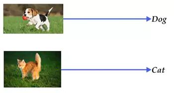
图1. 通用图像分类展示

图2展示了细粒度图像分类-花卉识别的效果，要求模型可以正确识别花的类别。

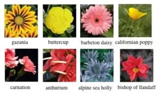
图2. 细粒度图像分类展示

一个好的模型既要对不同类别识别正确，同时也应该能够对不同视角、光照、背景、变形或部分遮挡的图像正确识别(这里我们统一称作图像扰动)。图3展示了一些图像的扰动，较好的模型会像聪明的人类一样能够正确识别。

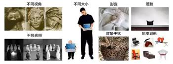
图3. 扰动图片展示[7]

模型概览：CNN

传统CNN包含卷积层、全连接层等组件，并采用softmax多类别分类器和多类交叉熵损失函数，一个典型的卷积神经网络如图4所示，我们先介绍用来构造CNN的常见组件。

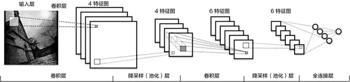
图4. CNN网络示例[5]

• 卷积层(convolution layer): 执行卷积操作提取底层到高层的特征，发掘出图片局部关联性质和空间不变性质。

• 池化层(pooling layer): 执行降采样操作。通过取卷积输出特征图中局部区块的最大值(max-pooling)或者均值(avg-pooling)。降采样也是图像处理中常见的一种操作，可以过滤掉一些不重要的高频信息。

• 全连接层(fully-connected layer，或者fc layer): 输入层到隐藏层的神经元是全部连接的。

• 非线性变化: 卷积层、全连接层后面一般都会接非线性变化函数，例如Sigmoid、Tanh、ReLu等来增强网络的表达能力，在CNN里最常使用的为ReLu激活函数。

• Dropout [1] : 在模型训练阶段随机让一些隐层节点权重不工作，提高网络的泛化能力，一定程度上防止过拟合。

接下来我们主要介绍VGG，ResNet网络结构。

1、VGG

牛津大学VGG(Visual Geometry Group)组在2014年ILSVRC提出的模型被称作VGG模型[2] 。该模型相比以往模型进一步加宽和加深了网络结构，它的核心是五组卷积操作，每两组之间做Max-Pooling空间降维。同一组内采用多次连续的3X3卷积，卷积核的数目由较浅组的64增多到最深组的512，同一组内的卷积核数目是一样的。卷积之后接两层全连接层，之后是分类层。由于每组内卷积层的不同，有11、13、16、19层这几种模型，下图展示一个16层的网络结构。

VGG模型结构相对简洁，提出之后也有很多文章基于此模型进行研究，如在ImageNet上首次公开超过人眼识别的模型[4]就是借鉴VGG模型的结构。

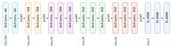
图5. 基于ImageNet的VGG16模型

2、ResNet

ResNet(Residual Network) [3] 是2015年ImageNet图像分类、图像物体定位和图像物体检测比赛的冠军。针对随着网络训练加深导致准确度下降的问题，ResNet提出了残差学习方法来减轻训练深层网络的困难。在已有设计思路(BN, 小卷积核，全卷积网络)的基础上，引入了残差模块。每个残差模块包含两条路径，其中一条路径是输入特征的直连通路，另一条路径对该特征做两到三次卷积操作得到该特征的残差，最后再将两条路径上的特征相加。

残差模块如图7所示，左边是基本模块连接方式，由两个输出通道数相同的3×3卷积组成。右边是瓶颈模块(Bottleneck)连接方式，之所以称为瓶颈，是因为上面的1×1卷积用来降维(图示例即256->64)，下面的1×1卷积用来升维(图示例即64->256)，这样中间3×3卷积的输入和输出通道数都较小(图示例即64->64)。

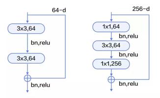
图7. 残差模块

3、数据准备

由于ImageNet数据集较大，下载和训练较慢，为了方便大家学习，我们使用CIFAR10数据集。CIFAR10数据集包含60,000张32×32的彩色图片，10个类别，每个类包含6,000张。其中50,000张图片作为训练集，10000张作为测试集。图11从每个类别中随机抽取了10张图片，展示了所有的类别。

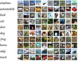
图11. CIFAR10数据集[6]

Paddle API提供了自动加载cifar数据集模块paddle.dataset.cifar。

通过输入python train.py，就可以开始训练模型了，以下小节将详细介绍train.py的相关内容。

模型结构

1、Paddle 初始化

让我们从导入Paddle Fluid API 和辅助模块开始。

from __future__ import print_function
import os
import paddle
import paddle.fluidas fluid
import numpy
import sys
from vgg import vgg_bn_drop
from resnet import resnet_cifar10

本教程中我们提供了VGG和ResNet两个模型的配置。

2、VGG

首先介绍VGG模型结构，由于CIFAR10图片大小和数量相比ImageNet数据小很多，因此这里的模型针对CIFAR10数据做了一定的适配。卷积部分引入了BN和Dropout操作。VGG核心模块的输入是数据层，vgg_bn_drop定义了16层VGG结构，每层卷积后面引入BN层和Dropout层，详细的定义如下：

def vgg_bn_drop(input):
def conv_block(ipt, num_filter, groups, dropouts):
return fluid.nets.img_conv_group(
input=ipt,
pool_size=2,
pool_stride=2,
conv_num_filter=[num_filter] * groups,
conv_filter_size=3,
conv_act=’relu’,
conv_with_batchnorm=True,
conv_batchnorm_drop_rate=dropouts,
pool_type=’max’)
conv1= conv_block(input, 64, 2, [0.3, 0])
conv2= conv_block(conv1, 128, 2, [0.4, 0])
conv3= conv_block(conv2, 256, 3, [0.4, 0.4, 0])
conv4= conv_block(conv3, 512, 3, [0.4, 0.4, 0])
conv5= conv_block(conv4, 512, 3, [0.4, 0.4, 0])
drop= fluid.layers.dropout(x=conv5, dropout_prob=0.5)
fc1= fluid.layers.fc(input=drop, size=512, act=None)
bn= fluid.layers.batch_norm(input=fc1, act=’relu’)
drop2= fluid.layers.dropout(x=bn, dropout_prob=0.5)
fc2= fluid.layers.fc(input=drop2, size=512, act=None)
predict= fluid.layers.fc(input=fc2, size=10, act=’softmax’)
return predict

首先定义了一组卷积网络，即conv_block。卷积核大小为3×3，池化窗口大小为2×2，窗口滑动大小为2，groups决定每组VGG模块是几次连续的卷积操作，dropouts指定Dropout操作的概率。所使用的img_conv_group是在paddle.fluit.net中预定义的模块，由若干组Conv->BN->ReLu->Dropout 和一组Pooling 组成。

五组卷积操作，即5个conv_block。第一、二组采用两次连续的卷积操作。第三、四、五组采用三次连续的卷积操作。每组最后一个卷积后面Dropout概率为0，即不使用Dropout操作。

最后接两层512维的全连接。

在这里，VGG网络首先提取高层特征，随后在全连接层中将其映射到和类别维度大小一致的向量上，最后通过Softmax方法计算图片划为每个类别的概率。

3、ResNet

ResNet模型的第1、3、4步和VGG模型相同，这里不再介绍。主要介绍第2步即CIFAR10数据集上ResNet核心模块。

先介绍resnet_cifar10中的一些基本函数，再介绍网络连接过程。

• conv_bn_layer: 带BN的卷积层。

• shortcut: 残差模块的”直连”路径，”直连”实际分两种形式：残差模块输入和输出特征通道数不等时，采用1×1卷积的升维操作；残差模块输入和输出通道相等时，采用直连操作。

• basicblock: 一个基础残差模块，即图9左边所示，由两组3×3卷积组成的路径和一条”直连”路径组成。

• layer_warp: 一组残差模块，由若干个残差模块堆积而成。每组中第一个残差模块滑动窗口大小与其他可以不同，以用来减少特征图在垂直和水平方向的大小。

def conv_bn_layer(input,
ch_out,
filter_size,
stride,
padding,
act=’relu’,
bias_attr=False):
tmp= fluid.layers.conv2d(
input=input,
filter_size=filter_size,
num_filters=ch_out,
stride=stride,
padding=padding,
act=None,
bias_attr=bias_attr)
return fluid.layers.batch_norm(input=tmp, act=act)
def shortcut(input, ch_in, ch_out, stride):
if ch_in!= ch_out:
return conv_bn_layer(input, ch_out, 1, stride, 0, None)
else:
return input
def basicblock(input, ch_in, ch_out, stride):
tmp= conv_bn_layer(input, ch_out, 3, stride, 1)
tmp= conv_bn_layer(tmp, ch_out, 3, 1, 1, act=None, bias_attr=True)
short= shortcut(input, ch_in, ch_out, stride)
return fluid.layers.elementwise_add(x=tmp, y=short, act=’relu’)
def layer_warp(block_func, input, ch_in, ch_out, count, stride):
tmp= block_func(input, ch_in, ch_out, stride)
for iin range(1, count):
tmp= block_func(tmp, ch_out, ch_out, 1)
return tmp

resnet_cifar10的连接结构主要有以下几个过程。

底层输入连接一层conv_bn_layer，即带BN的卷积层。

然后连接3组残差模块即下面配置3组layer_warp，每组采用图10 左边残差模块组成。

最后对网络做均值池化并返回该层。

注意：除第一层卷积层和最后一层全连接层之外，要求三组layer_warp总的含参层数能够被6整除，即resnet_cifar10的depth 要满足(depth – 2) % 6 = 0

def resnet_cifar10(ipt, depth=32):
# depth should be one of 20, 32, 44, 56, 110, 1202
assert (depth- 2) % 6== 0
n= (depth- 2) // 6
nStages= {16, 64, 128}
conv1= conv_bn_layer(ipt, ch_out=16, filter_size=3, stride=1, padding=1)
res1= layer_warp(basicblock, conv1, 16, 16, n, 1)
res2= layer_warp(basicblock, res1, 16, 32, n, 2)
res3= layer_warp(basicblock, res2, 32, 64, n, 2)
pool= fluid.layers.pool2d(
input=res3, pool_size=8, pool_type=’avg’, pool_stride=1)
predict= fluid.layers.fc(input=pool, size=10, act=’softmax’)
return predict

4、Infererence配置

网络输入定义为data_layer(数据层)，在图像分类中即为图像像素信息。CIFRAR10是RGB 3通道32×32大小的彩色图，因此输入数据大小为3072(3x32x32)。

def inference_network():
# The image is 32 * 32 with RGB representation.
data_shape = [3, 32, 32]
images = fluid.layers.data(name=’pixel’, shape=data_shape, dtype=’float32’)
predict = resnet_cifar10(images, 32)
# predict = vgg_bn_drop(images) # ment to use vgg net
return predict

5、Train 配置

然后我们需要设置训练程序train_network。它首先从推理程序中进行预测。在训练期间，它将从预测中计算avg_cost。在有监督训练中需要输入图像对应的类别信息，同样通过fluid.layers.data来定义。训练中采用多类交叉熵作为损失函数，并作为网络的输出，预测阶段定义网络的输出为分类器得到的概率信息。

注意:训练程序应该返回一个数组，第一个返回参数必须是avg_cost。训练器使用它来计算梯度。

def train_network(predict):
label = fluid.layers.data(name=’label’, shape=[1], dtype=’int64’)
cost = fluid.layers.cross_entropy(input=predict, label=label)
avg_cost = fluid.layers.mean(cost)
accuracy = fluid.layers.accuracy(input=predict, label=label)
return [avg_cost, accuracy]

6、Optimizer 配置

在下面的Adam optimizer，learning_rate是学习率，与网络的训练收敛速度有关系。

def optimizer_program():
return fluid.optimizer.Adam(learning_rate=0.001)

7、训练模型

-1）Data Feeders 配置

cifar.train10()每次产生一条样本，在完成shuffle和batch之后，作为训练的输入。

# Each batch will yield 128 images
BATCH_SIZE= 128
# Reader for training
train_reader = paddle.batch(
paddle.reader.shuffle(
paddle.dataset.cifar.train10(), buf_size=128 * 100),
batch_size=BATCH_SIZE)
# Reader for testing. A separated data set for testing.
test_reader = paddle.batch(
paddle.dataset.cifar.test10(), batch_size=BATCH_SIZE)

-2）Trainer 程序的实现

我们需要为训练过程制定一个main_program, 同样的，还需要为测试程序配置一个test_program。定义训练的place，并使用先前定义的优化器。

place = fluid.CUDAPlace(0) if use_cuda else fluid.CPUPlace()
feed_order = [’pixel’, ’label’]
main_program = fluid.default_main_program()
star_program = fluid.default_startup_program()
predict = inference_network()
avg_cost, acc = train_network(predict)
# Test program
test_program = main_program.clone(for_test=True)
optimizer = optimizer_program()
optimizer.minimize(avg_cost)
exe = fluid.Executor(place)
EPOCH_NUM = 1
# For training test cost
def train_test(program, reader):
count = 0
feed_var_list = [
program.global_block().var(var_name) for var_name in feed_order
]
feeder_test = fluid.DataFeeder(feed_list=feed_var_list, place=place)
test_exe = fluid.Executor(place)
accumulated = len([avg_cost, acc]) * [0]
for tid, test_data in enumerate(reader()):
avg_cost_np = test_exe.run(
program=program,
feed=feeder_test.feed(test_data),
fetch_list=[avg_cost, acc])
accumulated = [
x[0] + x[1][0] for x in zip(accumulated, avg_cost_np)
]
count += 1
return [x / count for x in accumulated]

-3）训练主循环以及过程输出

在接下来的主训练循环中，我们将通过输出来来观察训练过程，或进行测试等。

# main train loop.
def train_loop():
feed_var_list_loop = [
main_program.global_block().var(var_name) for var_name in feed_order
]
feeder = fluid.DataFeeder(feed_list=feed_var_list_loop, place=place)
exe.run(star_program)
step = 0
for pass_id in range(EPOCH_NUM):
for step_id, data_train in enumerate(train_reader()):
avg_loss_value = exe.run(
main_program,
feed=feeder.feed(data_train),
fetch_list=[avg_cost, acc])
if step_id % 100 == 0:
print(”
Pass %d, Batch %d, Cost %f, Acc %f” % (
step_id, pass_id, avg_loss_value[0], avg_loss_value[1]))
else:
sys.stdout.write(’.’)
sys.stdout.flush()
step += 1
avg_cost_test, accuracy_test = train_test(
test_program, reader=test_reader)
print(’
Test with Pass {0}, Loss {1:2.2}, Acc {2:2.2}’.format(
pass_id, avg_cost_test, accuracy_test))
if params_dirname is not None:
fluid.io.save_inference_model(params_dirname, [“pixel”],
[predict], exe)
train_loop()

-4）训练

通过trainer_loop函数训练, 这里我们只进行了2个Epoch, 一般我们在实际应用上会执行上百个以上Epoch

注意:CPU，每个Epoch 将花费大约15～20分钟。这部分可能需要一段时间。请随意修改代码，在GPU上运行测试，以提高训练速度。

train_loop()

一轮训练log示例如下所示，经过1个pass，训练集上平均Accuracy 为0.59 ，测试集上平均Accuracy 为0.6 。

Pass 0, Batch 0, Cost 3.869598, Acc 0.164062

………………………………………………………………………………………

Pass 100, Batch 0, Cost 1.481038, Acc 0.460938

………………………………………………………………………………………

Pass 200, Batch 0, Cost 1.340323, Acc 0.523438

………………………………………………………………………………………

Pass 300, Batch 0, Cost 1.223424, Acc 0.593750

………………………………………………………………………………

Test with Pass 0, Loss 1.1, Acc 0.6

图13是训练的分类错误率曲线图，运行到第200个pass后基本收敛，最终得到测试集上分类错误率为8.54%。

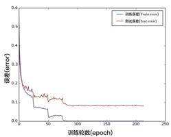
图13. CIFAR10数据集上VGG模型的分类错误率

应用模型

可以使用训练好的模型对图片进行分类，下面程序展示了如何加载已经训练好的网络和参数进行推断。

1、生成预测输入数据

dog.png是一张小狗的图片. 我们将它转换成numpy数组以满足feeder的格式.

from PIL import Image
def load_image(infer_file):
im = Image.open(infer_file)
im = im.resize((32, 32), Image.ANTIALIAS)
im = numpy.array(im).astype(numpy.float32)
# The storage order of the loaded image is W(width),
# H(height), C(channel). PaddlePaddle requires
# the CHW order, so transpose them.
im = im.transpose((2, 0, 1)) # CHW
im = im / 255.0
# Add one dimension to mimic the list format.
im = numpy.expand_dims(im, axis=0)
return im
cur_dir = os.path.dirname(os.path.realpath(__file__))
img = load_image(cur_dir + ’/image/dog.png’)

2、Inferencer 配置和预测

与训练过程类似，inferencer需要构建相应的过程。我们从params_dirname加载网络和经过训练的参数。我们可以简单地插入前面定义的推理程序。现在我们准备做预测。

place = fluid.CUDAPlace(0) if use_cuda else fluid.CPUPlace()
exe = fluid.Executor(place)
inference_scope = fluid.core.Scope()
with fluid.scope_guard(inference_scope):
# Use fluid.io.load_inference_model to obtain the inference program desc,
# the feed_target_names (the names of variables that will be feeded
# data using feed operators), and the fetch_targets (variables that
# we want to obtain data from using fetch operators).
[inference_program, feed_target_names,
fetch_targets] = fluid.io.load_inference_model(params_dirname, exe)
# The input’s dimension of conv should be 4-D or 5-D.
# Use inference_transpiler to speedup
inference_transpiler_program = inference_program.clone()
t = fluid.transpiler.InferenceTranspiler()
t.transpile(inference_transpiler_program, place)
# Construct feed as a dictionary of {feed_target_name: feed_target_data}
# and results will contain a list of data corresponding to fetch_targets.
results = exe.run(
inference_program,
feed={feed_target_names[0]: img},
fetch_list=fetch_targets)
transpiler_results = exe.run(
inference_transpiler_program,
feed={feed_target_names[0]: img},
fetch_list=fetch_targets)
assert len(results[0]) == len(transpiler_results[0])
for i in range(len(results[0])):
numpy.testing.assert_almost_equal(
results[0][i], transpiler_results[0][i], decimal=5)
# infer label
label_list = [
“airplane”, “automobile”, “bird”, “cat”, “deer”, “dog”, “frog”,
“horse”, “ship”, “truck”
]
print(“infer results: %s” % label_list[numpy.argmax(results[0])])

总结

传统图像分类方法由多个阶段构成，框架较为复杂，而端到端的CNN模型结构可一步到位，而且大幅度提升了分类准确率。本文我们首先介绍VGG、ResNet两个经典的模型；然后基于CIFAR10数据集，介绍如何使用PaddlePaddle配置和训练CNN模型；最后介绍如何使用PaddlePaddle的API接口对图片进行预测和特征提取。对于其他数据集比如ImageNet，配置和训练流程是同样的。请参照Github

https:///PaddlePaddle/models/blob/develop/PaddleCV/image_classification/.md。

参考文献

[1] G.E. Hinton, N. Srivastava, A. Krizhevsky, I. Sutskever, and R.R. Salakhutdinov. Improving neural networks by preventing co-adaptation of feature detectors. arXiv preprint arXiv:1207.0580, 2012.

[2] K. Chatfield, K. Simonyan, A. Vedaldi, A. Zisserman. Return of the Devil in the Details: Delving Deep into Convolutional Nets. BMVC, 2014。

[3] K. He, X. Zhang, S. Ren, J. Sun. Deep Residual Learning for Image Recognition. CVPR 2016.

[4] He, K., Zhang, X., Ren, S., and Sun, J. Delving Deep into Rectifiers: Surpassing Human-Level Performance on ImageNet Classification. ArXiv e-prints, February 2015.

[5] http://deeplearning.net/tutorial/lenet.html

[6] https://www.cs.toronto.edu/~kriz/cifar.html

[7] http://cs231n.github.io/classification/

以上就是关于gg游戏修改器教程贴吧_GG游戏修改器怎么使用的全部内容，游戏大佬们学会了吗？